Janai’s economics blog - Data analytics using Power BI

1 Introduction¹

In this month’s blog we touch on the data analytics software Power BI. Power BI is an analytics platform by Microsoft and allows for data analytics and data mining with relative ease. In the Caribbean region the tourism season is slowly winding down and I thought it best to speak on the industry but rather than touch on typical topics such as tourist arrivals and cruise passengers we can merge ongoing discussion surrounding data analytics, AI and tourism. How? The first component of this would be data, and the US Bureau of Transportation has a wealth of information which is publicly available. One of the datasets that ties into our looking into tourism this month is the International Report Passengers dataset. This dataset provides information such as carrier name, airport destination, flight origin and data from 1990 through to the end of 2023. This dataset therefore allows one to assess the behavior of US travelers and explore the extent to which any lessons of relevance can be found for the Caribbean region.

In this blog we’ll therefore:

Augment the Bureaus dataset with other information.
Explore the data cleaning and analysis process.
Review issues including discussing issues such as primary, foreign keys and fact tables.
Preliminary analysis of key trend and takeaways with a focus on reviewing what months do Americans travel the most, which destinations have seen the most growth, which are the most or least volatile and which areas in the USA are seeing the most change.

2 The Data

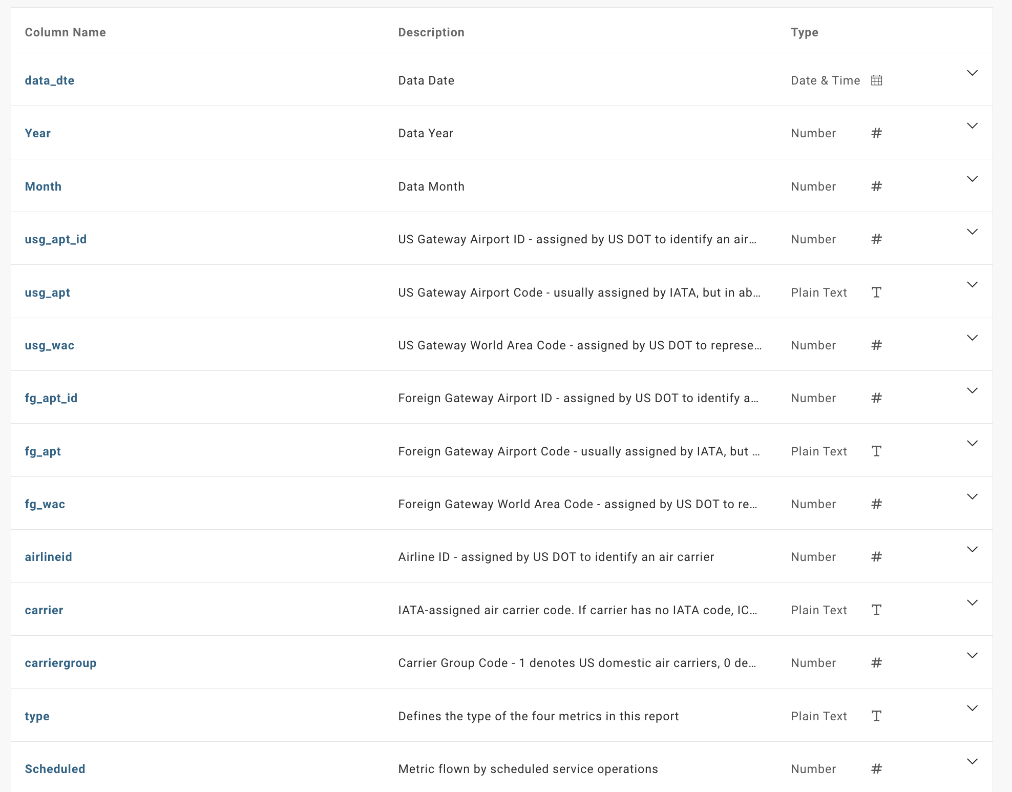
Our first port of call is reviewing the international passenger flow information. At first glance (see below) column names are unclear and most columns contain abbreviated codes and numbers such as LAX/MIA being used to describe airports see the field fg_apt and usg_apt.

Code

 glimpse(passenger_flows)

Rows: 774,489
Columns: 16
$ data_dte     <chr> "07/01/2004", "11/01/2008", "10/01/2002", "03/01/2007", "…
$ Year         <int> 2004, 2008, 2002, 2007, 2009, 2005, 2009, 2010, 2007, 200…
$ Month        <int> 7, 11, 10, 3, 3, 5, 4, 4, 2, 8, 11, 9, 7, 9, 9, 6, 10, 7,…
$ usg_apt_id   <int> 14747, 11697, 10257, 12889, 12892, 11298, 13303, 14843, 1…
$ usg_apt      <chr> "SEA", "FLL", "ALB", "LAS", "LAX", "DFW", "MIA", "SJU", "…
$ usg_wac      <int> 93, 33, 22, 85, 91, 74, 33, 3, 33, 21, 38, 33, 11, 22, 23…
$ fg_apt_id    <int> 16229, 12010, 16271, 13165, 13252, 10920, 14838, 13068, 1…
$ fg_apt       <chr> "YVR", "GUA", "YYZ", "MAN", "MEX", "CDG", "SJO", "LRM", "…
$ fg_wac       <int> 906, 127, 936, 493, 148, 427, 110, 224, 324, 493, 204, 11…
$ airlineid    <int> 19687, 20416, 20206, 19541, 19534, 19805, 19805, 20414, 1…
$ carrier      <chr> "QX", "NK", "QK", "BD", "AM", "AA", "AA", "OW", "AA", "CO…
$ carriergroup <int> 1, 1, 0, 0, 0, 1, 1, 1, 1, 1, 0, 1, 1, 0, 1, 0, 1, 0, 0, …
$ type         <chr> "Passengers", "Passengers", "Passengers", "Passengers", "…
$ Scheduled    <int> 19265, 3099, 33, 3815, 17993, 11530, 33400, 1383, 14056, …
$ Charter      <int> 0, 0, 0, 0, 0, 0, 0, 0, 0, 0, 0, 0, 0, 0, 0, 683, 0, 0, 0…
$ Total        <int> 19265, 3099, 33, 3815, 17993, 11530, 33400, 1383, 14056, …

Thankfully the US Bureau of Transportation provides a description of the data and we recognize that passenger flows (Scheduled, Charter, Total) are recorded for source airport (usg_apt) and destination airport (fg_apt) in addition to by date (data_dte) and carrier. Despite this clarification the obvious shortcoming of the information provided is that fields such as destination country, full airport names, US State and city of originating flight is not provided.

We can create these fields by leveraging other publicly available datasets of all airports and the respective countries and cities in addition to information of all airlines in the world. The availability of these datasets allows us to touch one of the key aspects of data analytics where there are multiple related data sources i.e. creating a data model.

3 The Data Model

Let’s therefore create a data model to better understand the flight data provided by the Bureau of Transportation. A data model is defined “as a model which organizes elements and standardizes how the data elements relate to one another”² . In our case well have five datasets which we’ll attempt to connect and join:

The passenger flows dataset,
A matrix of dates,
A table of all US airports by State, city and name,
A table of all international airports and their names ,
A table of Caribbean island names and
A table of all countries in the world.

A good explanation of how a data model is to look at the raw flight airport code data and envisage a situation where this can be instantly connected with full airport name and State and country. This intent allows us to touch on the concepts below:

Fact table: this stores quantitative information and will be connected to each of our dimension tables. In our case here we ll store the number of passengers per destination
Dimension tables: these are tables built on specific attributes which can relate to our fact table. In our example an example would be a table with all airlines names and codes, another would be a table with all airport names etc
Primary keys: these are unique identifiers in a table. In the dimension table with airline names we ll have a table with two columns one named “airline codes” with a column of values like AA or BA and another column with names such as American Airlines or British Airways. The column “airline code” would be a primary key for that table.
Foreign keys: building off the example above in our fact table which would have quantitative data on passenger flows we will have a column with airline codes lets assume its named “codes”. That column “codes” would be a foreign key column as it would establish a relationship with “airline code” in the aforementioned dimension table.

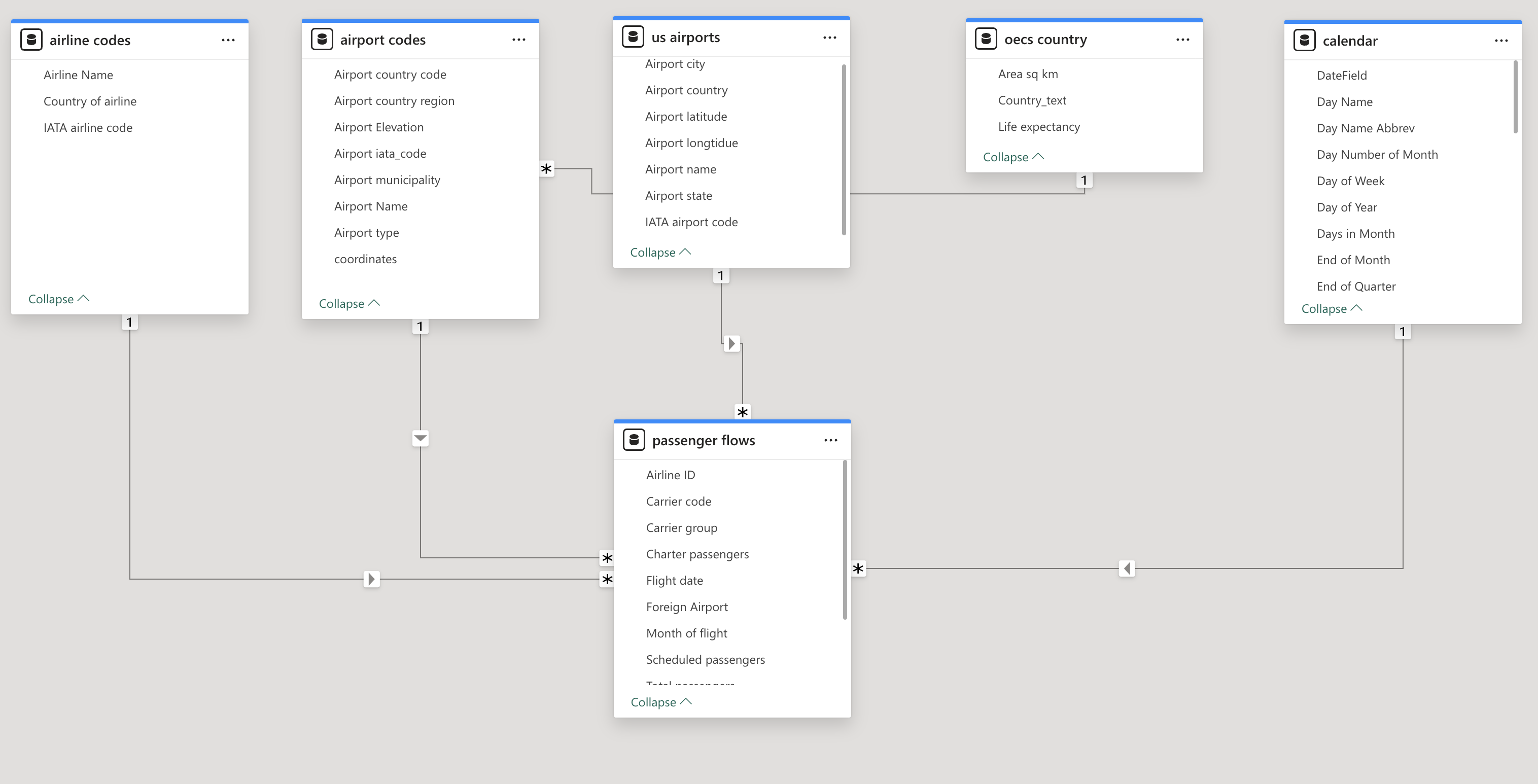
Using Power Bi we can connect these tables to create a data model³ below

In this data model we have connected (see the lines with arrows) five dimension tables to our fact table “passenger flows”. The connections made are:

Between the “airline codes” dimension table and the “passenger flows” fact table we have connected IATA airline code : carrier code,
Between the “airport codes” dimension table and the “passenger flows” fact table we have connected Airport IATA code : Foreign airport,
Between the “us airport” dimension table and the “passenger flows” fact table we have connected IATA airport code : US airport,
Between the “calender” dimension table and the “passenger flows” fact table we have connected the Date field : Flight date

To give some sense as to what the dimension tables look like lets have a look at the airline and airport code tables.

The airlines data looks like this:

Code

 glimpse(airlines)

Rows: 253
Columns: 5
$ `Airline Name`    <chr> "ABSA Cargo Airline", "Adria Airways", "Aegean Airli…
$ `IATA Designator` <chr> "M3", "JP", "A3", "EI", "P5", "SU", "AR", "2K", "AM"…
$ `3-Digit Code`    <chr> NA, "165", "390", "053", "845", "555", "044", "547",…
$ `ICAO Designator` <chr> "TUS", "ADR", "AEE", "EIN", "RBP", "AFL", "ARG", "54…
$ Country           <chr> "Brazil", "Slovenia", "Greece", "Ireland", "Colombia…

while the airports data looks like this

Code

 glimpse(airports)

Rows: 57,421
Columns: 12
$ ident        <chr> "00A", "00AA", "00AK", "00AL", "00AR", "00AS", "00AZ", "0…
$ type         <chr> "heliport", "small_airport", "small_airport", "small_airp…
$ name         <chr> "Total Rf Heliport", "Aero B Ranch Airport", "Lowell Fiel…
$ elevation_ft <int> 11, 3435, 450, 820, 237, 1100, 3810, 3038, 87, 3350, 4830…
$ continent    <chr> NA, NA, NA, NA, NA, NA, NA, NA, NA, NA, NA, NA, NA, NA, N…
$ iso_country  <chr> "US", "US", "US", "US", "US", "US", "US", "US", "US", "US…
$ iso_region   <chr> "US-PA", "US-KS", "US-AK", "US-AL", "US-AR", "US-OK", "US…
$ municipality <chr> "Bensalem", "Leoti", "Anchor Point", "Harvest", "Newport"…
$ gps_code     <chr> "00A", "00AA", "00AK", "00AL", "", "00AS", "00AZ", "00CA"…
$ iata_code    <chr> "", "", "", "", "", "", "", "", "", "", "", "", "", "", "…
$ local_code   <chr> "00A", "00AA", "00AK", "00AL", "", "00AS", "00AZ", "00CA"…
$ coordinates  <chr> "-74.93360137939453, 40.07080078125", "-101.473911, 38.70…

We can see that the airlines data shows the airline name and country while the airport file shows descriptions of airports including elevation, type and country code.

4 Analysis of the data model

Now that we have created the data model we can create a more intuitive and information table such as the one below:

This table shows what the full dataset looks like with all the relationships built in, note that we now have airlines names and destination countries. This however is a large dataset as shown by the number of rows at 774,489. We therefore create a truncated dataset of only CARICOM countries shown below.

Getting to this stage can be explained by the chart below where we were able to pull out the Caricom countries by doing an inner join of our full dataset and a list of Caricom countries of interest.

Note that our list of countries⁴ are:

Antigua and Barbuda
Barbados
Dominica
Grenada
Saint Lucia
St. Vincent and the Grenadines and
Trinidad and Tobago

5 Tables of US flows to the Caricom region

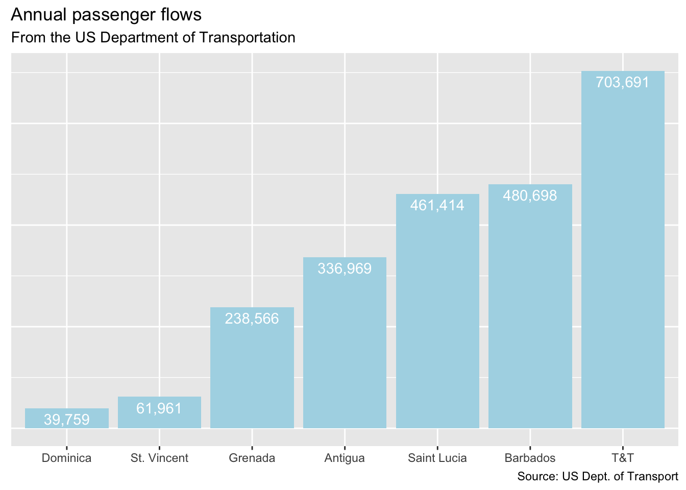
Now that we have our dataset lets work on building out a few tables and charts. The first chart we will build is one showing passenger flows to select Caribbean islands see Figure 1.

Figure 1: Annual US Arrivals in 2023 (select countries)

In Figure 1 we see that Barbados and Trinidad and Tobago have the largest flows in 2023, followed by Saint Lucia. We can do the same thing but this time for airlines.

Figure 2: Annual US Arrivals to Select Caribbean Countries in 2023

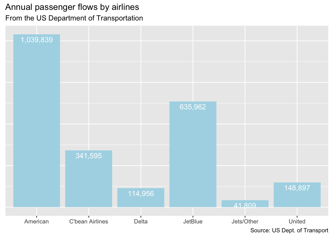
Where we can see from Figure 2 that American Airlines and Jet Blue are the largest carriers operating in the region in 2023.

We can also focus our attention on a particular country. Say Saint Lucia and assess passenger flows by US State and City. Here in Table 1 that Florida and New York are the largest hubs servicing the region.

Table 1:
Passenger flows to Saint Lucia
US State	City	Number of passengers
Passenger flows to Saint Lucia
by US State and City
Florida	Miami	130,868
New York	New York	123,368
Georgia	Atlanta	102,655
North Carolina	Charlotte	73,041
New Jersey	Newark	10,452
Pennsylvania	Philadelphia	7,164
Massachusetts	Boston	7,095
Illinois	Chicago	4,501
Puerto Rico	San Juan	1,544
Florida	Orlando	308
Texas	Dallas-Fort Worth	245
Florida	Ft. Lauderdale	151
Florida	West Palm Beach	12
California	Oakland	6
Virginia	Chantilly	4
Source: US Dept of Transport

6 Conclusion

We have seen that the International Report Passengers ⁵ dataset, with some data cleaning and analysis can provide insights into passenger flows to the Caribbean. We can assess flows by airline, US State, City and other characteristics when can be useful for benchmarking and other bits of analysis. This also shows the promise of business intelligence tools like Power BI and Tableau which can allow deep dives into data.

Footnotes

Photo by Eyosias G on Unsplash ↩︎
What is a Data Model? | Center for Data, Analytics and Reporting (princeton.edu)↩︎
Note that we have changed the column names in the passenger flow dataset to be more intuitive based on figure 1↩︎
Jamaica is excluded↩︎
The only downside is that there is a 6 month lag in the data set.↩︎

1 Introduction1

2 The Data

3 The Data Model

4 Analysis of the data model

5 Tables of US flows to the Caricom region

6 Conclusion

Footnotes

1 Introduction¹